Hopfield Network
Hopfield networks were introduced in 1982 by John Hopfield and they represent the return of Neural Networks to the Artificial Intelligence field. I will briefly explore its continuous version as a mean to understand Boltzmann Machines.
The Hopfield nets are mainly used as associative memories and for solving optimization problems. The associative memory links concepts by association, for example when you hear or see an image of the Eiffel Tower you might recall that it is in Paris.
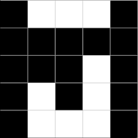
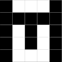
The inputs and outputs of the Hopfield network are binary, so we can train it to remember B&W images such as a collection of letters. For instance, we can teach them the next set of letters:
 |
 |
 |
 |
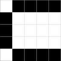
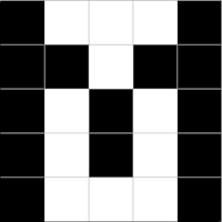
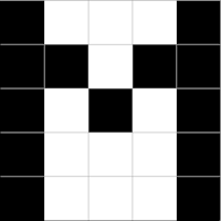
So how does the Hopfield network recalls a pattern? Well, the recalling process is iterative and in each cycle all the neurons in the net are fired. This process ends when the state of the neurons doesn’t change, as seen in the next figure.
(a) Input pattern
|
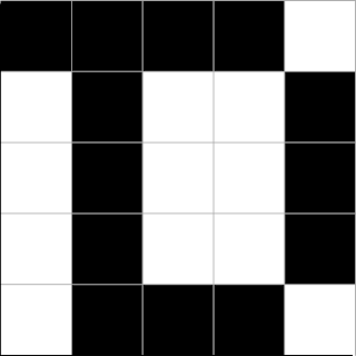
(b) Iteration 1
|
(c) Iteration 2
|
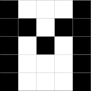
(d) Iteration 3
|
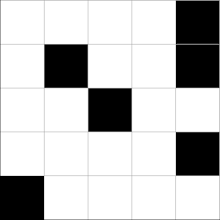
(e) Final iteration
|
Architecture
A Hopfield net is a set of neurons that are:
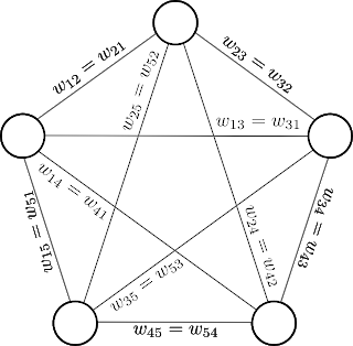
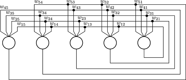
Both properties are illustrated in Fig. 3, where a Hopfield network consisting of 5 neurons is shown. One property that the diagram fails to capture it is the recurrency of the network. The Hopfield networks are recurrent because the inputs of each neuron are the outputs of the others, i.e. it posses feedback loops as seen in Fig. 4. This last property is better understood by the recalling process. |
|
|
Fig. 4. A Hopfield network consisting of 5 neurons with feedback loops. Based on Haykin.
|
Learning Rule
In order to learn a set of patterns \(\boldsymbol{x}^{(n)}\), such as the four letters presented above, the weights of the net must be set using the Hebb Rule:
\[w_{ij}=\eta\sum_n{x_{i}^{(n)}x_{j}^{(n)}}\]where \(\eta\) is a constant that might be set to \(\eta=1/N\) for \(N\) patterns. In the case of the continuous Hopfield network, this constant prevents the weight from growing with $N$. The idea of the Hebbian rule is that two neurons that are repeatedly fired at the same time must have a stronger association.
Activity Rule
The activation \(a_{i}\) of the neuron \(i\) is given by
\[a_{i}=\eta\sum_j{w_{ij}x_{j}}\]and the update of the state \(x_{i}\) for the continuous case is given by
\[x_{i}=\tanh{(a_{i})}\]The order of the neuron updates can be performed synchronously or asynchronously. In the former kind the activation and update of all neurons are done at the same time. In the latter kind the neurons are activated and updates sequentially and its order is randomly permuted beforehand.
Convergence
After seeing the recalling process example one might be wondering many interesting questions like does the Hopfield network will always stabilize? The answer is yes, but the net might not recall the correct pattern. This could happen if the net is overloaded or the weights were altered.
The convergence to a stable state is guaranteed for networks that have the two main characteristics of its architecture and that follows an asynchronous update procedure.
Please note that in this post I didn’t provide any mathematical proof for the convergence neither I talked about attractors, nonlinear dynamical systems, and Lyapunov functions. Maybe I will talk about them in a future post, in the meantime please see the references section.
Code
I provide the implementation of the example I presented, which originally appeared in MacKay. I tried to make it as small as possible and hoping to be useful.
import numpy as np
import matplotlib.pyplot as plt
import matplotlib.lines as mlines
import matplotlib.patches as mpatches

def plotLetter(letter):
    black = '#000000'; white='#FFFFFF'; gray='#AAAAAA'
    squareSide = 0.03

    plt.figure(figsize=(5,5))
    ax = plt.axes([0,0,6.5,6.5])

    # Plotting squares
    for i in xrange(25):
        coords = np.array([i%5*squareSide, (4-i/5)*squareSide])
        color = black if letter[i]< 0 else white
        square = mpatches.Rectangle(coords, squareSide, squareSide,
                                                      color = color, linewidth=0.5)
        ax.add_patch(square)

    # Plotting grid
    for i in xrange(6):
        x = (5-i%5)*squareSide
        s1, s2 = np.array([[x, x], [0, 5*squareSide]])
        ax.add_line(mlines.Line2D(s1, s2, lw=1, color = gray ))
        ax.add_line(mlines.Line2D(s2, s1, lw=1, color = gray ))

patterns = np.array([
   [-1,-1,-1,-1,1,1,-1,1,1,-1,1,-1,1,1,-1,1,-1,1,1,-1,1,-1,-1,-1,1.],   # Letter D
   [-1,-1,-1,-1,-1,1,1,1,-1,1,1,1,1,-1,1,-1,1,1,-1,1,-1,-1,-1,1,1.],    # Letter J
   [1,-1,-1,-1,-1,-1,1,1,1,1,-1,1,1,1,1,-1,1,1,1,1,1,-1,-1,-1,-1.],     # Letter C
   [-1,1,1,1,-1,-1,-1,1,-1,-1,-1,1,-1,1,-1,-1,1,1,1,-1,-1,1,1,1,-1.],], # Letter M
   dtype=np.float)

n = patterns.shape[0]
m = patterns.shape[1]
eta = 1./n

# training
weights = np.zeros((m,m))
for i in xrange(m-1):
    for j in xrange(i+1,m):
        weights[i,j] = eta*np.dot(patterns[:,i], patterns[:,j])
        weights[j,i] = weights[i,j]

activations = np.zeros(m)
states = np.array([1,1,1,1,-1,1,-1,1,1,-1,1,1,-1,1,1,1,1,1,1,-1,-1,1,1,1,1],
                   dtype=np.float)
plotLetter(states)

# recalling
np.random.seed(10)
for itr in range(4):
    for i in np.random.permutation(m): # asynchronous activation
        activations[i] = np.dot(weights[i,:], states)
        states[i]=np.tanh(activations[i])
    plotLetter(states)
plt.show()
References
I heavily used the book Information Theory, Inference and Learning Algorithms by David MacKay for writing this post. The example presented in this post is discussed in depth in the same book. Another good source for understanding the training and update procedures is presented in this page. By the way, David MacKay is one of Hopfield’s PhD alumni.
I also found useful these books NeuralNetworks and Learning Machines, Bayesian Reasoning and Machine Learning, and Neural Networks - A Systematic Introduction. Another resources on the web are wikipedia and scholarpedia.
In the next post I will provide a fairly common example of Gibbs sampling in Python and give a brief explanation.