Simulated Annealing

Simulated annealing is a meta-algorithm used for solving optimization problems. It is based on the annealing process that consists in heating a metal or a glass and then cooling it slowly. The purpose of this procedure is to remove internal stresses and toughen it. A more formal definition relies on Thermodynamics and it greatly helps to understand the algorithm.

Annealing

The objective of annealing is to make a metal or a glass tougher o more resistant. The level of resistance of a material depends on its crystal structure, which defines a tridimensional pattern of positions for its electrons. For example, an easy breakable sword might contain more than one crystal structures that could be fragmented in a single hit.

When a metal is heated up to its melting point, its electron are highly excited and they move randomly across the material. At this point, the electrons form many configurations of crystal structures. A crystal structure that has a few contacts between electrons is said to possess a high energy level or state. When the temperature is slowly cool, the electrons lose mobility and the energy state gets lower and lower. This means that the electrons gain more and more contacts with each other.

Finally, when the temperature settles down the electrons reach a single lattice in which they have the most possible contacts with each other. In other words, they have reach a global energy minimum and we obtain a flexible and resistant sword.

The Boltzmann Distribution Law

The Boltzmann distribution law describes the probability $p_j$ of a thermodynamic system being at a particular state $E_j$ at some temperature $T$ in equilibrium. It is stated as follows:

\[\begin{equation} p_j=\frac{e^{-E_j/kT}}{\displaystyle\sum_{j=1}^{t}e^{-E_j/kT}}=\frac{e^{-E_j/kT}}{Q} \end{equation}\]

where $t$ is the number of possible states, $k$ refers to the Boltzmann’s constant equal to 1.380662 x $10^{-23}$ joules/kelvin and $Q$ is the partition function. The Boltzmann distribution basically says that at high temperatures the probability of occurrence of all states is higher than at lower temperatures. At low temperatures, the occurrence of all the states is possible, but the probability of occurrence is concentrated in states of low energy.

In fields other than Physics, the value of $k$ is usually set to 1 since the original value is suitable for units that only describe energy. Additionally, the partition function $Q$ can’t be always calculated and an approximation is used. In particular, for simulated annealing we employ the relative populations of particles in states $i$ and $j$ given by

\[\begin{equation} \frac{p_i}{p_j}=e^{-(E_i-E_j)/kT} \end{equation}\]

then taking $k=1$

\[\begin{equation} \frac{p_i}{p_j}=e^{-(E_i-E_j)/T} \end{equation}\]

Algorithm

The objective of simulated annealing is to find the global minimum of a function limited by lower and upper boundaries. The algorithm takes guesses of the function in a similar way of the annealing procedure. All the points contained within the function boundaries represent all possible electron states and the function to minimize represents the energy function.

Basically, simulated annealing is a random walk search plus a random control guidance. In a random walk search we sequentially take random points or states and we keep track of the state with the lowest energy. The randomness of the search will keep us out from local minima, but we need to exhaustively sample a lot of states in order to find the global energy minimum.

The pseudo temperature gives to our random walk a control guidance. Instead of jumping around from one state to another without any criteria, we will only jump if the next state has a lower energy or jump according to the probability given by the Boltzmann distribution. The former condition will improve the accuracy of our search and the latter will take us from local minima. So now we can consider a random walk search as a simulated annealing minimisation at a constant infinite temperature.

The following pseudocode presents the simulated annealing using a heuristic that keeps the best energy state, this listing is based on the one from wikipedia.

Input: initialState, energyFunction, boundaries, iterationMax, initialTemperature
Output: bestState, bestEnergy
   
    currentTemperature = initialTemperature
    currentState = initialState
    currentEnergy = energyFunction(currentState)
    
    bestState = currentState
    bestEnergy = currentEnergy
       
    for i = 1 to iterationMax:
        newState = createNeighbourSolution(boundaries, currentState)        
        newEnergy = energyOf(newState);
        deltaEnergy = newEnergy- currentEnergy;
            
        if deltaEnergy < 0
            state = newState;
            energy = newEnergy
            if newEnergy < bestEnergy:
             bestState = newState
         bestEnergy = newEnergy
        else if U[0,1] < exp(-deltaEnergy/currentTemperature)
            state = newState;
            energy = newEnergy;
           
        currentTemperature = calculateTemperature(i, currentTemperature)
return bestState, bestEnergy

Example

The objective of this example is to optimize the function

\[\begin{equation} f(x,y) = \frac{-\cos(\pi x)\cdot \cos(2\pi y)}{1+x^2+y^2} \end{equation}\]

where $x$ and $y \in [-1.75, 1.75]$. The plot of this function is shown in the next figure.

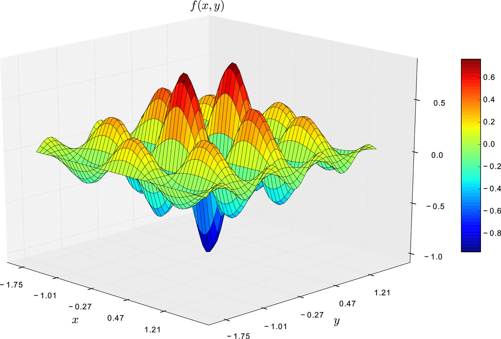
From the image above, it is clear that the global minimum is -1 and it is on state (0,0). Additionally, we can observe that the function has several local minima states, and first order optimisation methods might get stuck on them.

The function $f(x,y)$ will be the energy function to minimize with lower and upper boundaries set on -1.75 and 1.75 for both $x$ and $y$, respectively. Moreover, my function to create a random neighbour solution will simply be

\[\begin{equation} createNeighbourSolution(x,y) = \frac{upperBoundary-lowerBoundary}{2}\cdot\begin{pmatrix} U[-1,1]\\ U[-1,1] \end{pmatrix}+\begin{pmatrix} x\\ y \end{pmatrix} \end{equation}\]

where $createNeighbourSolution(x,y) \in [-1.75, 1.75]$.

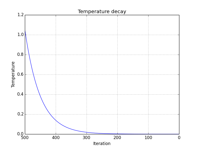
The function to calculate the temperature for each iteration $i$ is

\[\begin{equation} calculateTemperature(i, currentTemperature) = \alpha \cdot currentTemperature \end{equation}\]

where the constant $\alpha=0.98$ and the initial temperature is 1.05. A plot of the the temperature decay is shown below.

The only thing missing is to show the process of the simulated annealing. The next figure shows the contour plot of our energy function and the accepted and random states taken in the process. The star shows the best energy so far at each state. In this example, the initial state is set on purpose on $(0, 0.5)$, a local minimum point.

Code

The code for generating the example was pretty huge, so I decided to split the plots in three scripts. The script for plotting the three-dimensional energy function of the example is the next one.

from __future__ import division

import numpy as np
import matplotlib.cm as cm
import matplotlib.pyplot as plt
import mpl_toolkits.mplot3d

delta = 0.075
x = np.arange(-1.75, 1.75, delta)
y = np.arange(-1.75, 1.75, delta)
X, Y = np.meshgrid(x, y)
Z=(-np.cos(np.pi*(X))*np.cos(2*np.pi*(Y)))/ ( 1 +np.power(X,2) +np.power(Y,2))

fig = plt.figure()
ax = fig.gca(projection='3d')
fig.tight_layout()
ax.set_zlim(-1.05, 0.85)
ax.view_init(elev=20., azim=-45)
ax.set_aspect(0.75)
surf = ax.plot_surface(X, Y, Z, rstride=1, cstride=1, 
                       cmap=cm.jet, linewidth=0.5, antialiased=False)
fig.colorbar(surf, shrink=0.5, aspect=10)
plt.xticks(np.arange(min(x), max(x), 0.74))
plt.yticks(np.arange(min(y), max(y), 0.74))
plt.xlabel(r'x')
plt.ylabel(r'y')
plt.title(r'f(x,y)')
plt.show()

The script for plotting the temperature decay is.

import numpy as np
import matplotlib.pyplot as plt
alpha=0.98
temperature = alpha*np.ones((500,1))
temperature[0]=1.05
temperature = np.cumprod(temperature)

iteration = range(500,0,-1)

fig = plt.figure()
plt.plot(iteration,temperature)
plt.xlabel('Iteration')
plt.ylabel('Temperature')
plt.title('Temperature decay')

ax = fig.gca()
ax.set_xlim(ax.get_xlim()[::-1])

plt.grid(True)
plt.show()

Finally, the code for doing the simulated annealing is below. As you can see, most of the code is dedicated for doing the animated plot (lines 65-131) rather than the simulated annealing (lines 9-64).

from __future__ import division

import numpy as np
import matplotlib
import matplotlib.animation as animation
import matplotlib.pyplot as plt

def neighbour(upperBoundary, lowerBoundary, state): 
    deltaState = (2*np.random.random(state.shape)-1)*(upperBoundary-lowerBoundary)/2;
    newState = state + deltaState;
    newState = (newState < lowerBoundary)*lowerBoundary + \
                       (upperBoundary < newState)*upperBoundary+ \
                       (lowerBoundary <= newState)*(newState <= upperBoundary)*newState;                    
    return newState

def anneal(initialState, energyOf, lowerBoundary, upperBoundary, \
                   temperature, alpha, kMax):
    
    states = np.zeros((kMax+1,2))
    newStates = np.zeros((kMax+1,2))
    bestStates = np.zeros((kMax+1,2))
    bestEnergies = np.zeros(kMax+1)
    
    state = initialState;  energy = energyOf(initialState)
    bestState = initialState; bestEnergy = energy
        
    states[0,:] = initialState; newStates[0,:] = initialState
    bestStates[0,:] = initialState; bestEnergies[0] = bestEnergy
    i = 1

    for k in reversed(xrange(kMax)):
        newState = neighbour(upperBoundary, lowerBoundary, state)
        newEnergy = energyOf(newState);
        deltaEnergy = newEnergy- energy;
            
        if deltaEnergy < 0:
            state = newState;
            energy = newEnergy;
            if newEnergy < bestEnergy:
                bestState = newState
                bestEnergy = newEnergy
        elif np.random.uniform() < np.exp(-deltaEnergy/temperature):
            state = newState;
            energy = newEnergy;
                            
        temperature = alpha*temperature
                    
        states[i,:] = state; newStates[i,:] = newState
        bestStates[i,:] = bestState; bestEnergies[i] = bestEnergy  
        i+=1
    return bestState, bestEnergy, states, newStates, bestStates, bestEnergies

energyOf = lambda s: (-np.cos(np.pi*s[0])*np.cos(2*np.pi*s[1]))/ \
                                    (1+np.power(s,2).sum())
lowerBoundary = np.array([-1.75,-1.75], dtype=np.float)
upperBoundary = np.array([1.75,1.75], dtype=np.float)

initialState = np.array([0., 0.5], dtype=np.float)

temperature = 1.05
alpha = 0.98
kMax = 500

np.random.seed(20)    
bestState, bestEnergy, states, newStates, bestStates, bestEnergies = \
   anneal(initialState, energyOf, lowerBoundary, upperBoundary, \
               temperature, alpha, kMax)


# Animation plotting
delta = 0.075
x = np.arange(-1.85, 1.85, delta)
y = np.arange(-1.85, 1.85, delta)
X, Y = np.meshgrid(x, y)
Z=(-np.cos(np.pi*(X))*np.cos(2*np.pi*(Y)))/ ( 1 +np.power(X,2) +np.power(Y,2))

matplotlib.rcParams['xtick.direction'] = 'out'
matplotlib.rcParams['ytick.direction'] = 'out'
 
fig, (ax1, ax2) = plt.subplots(1, 2, sharey=True, figsize=(14,7))
ax1.set_title('Accepted states',fontweight='bold', fontsize=15)
ax1.set_xlabel('x')
ax1.set_ylabel('y')

ax2.set_title('Random states',fontweight='bold', fontsize=15)
ax2.set_xlabel('x')
 
contour = ax1.contour(X, Y, Z, linewidth = 5)
plt.clabel(contour, inline=1, fontsize=8)
 
contour = ax2.contour(X, Y, Z, linewidth = 5)
plt.clabel(contour, inline=1, fontsize=8)
 
ax1.grid()
ax2.grid()

fig.subplots_adjust(bottom=0.12)

iterNumLabel = plt.figtext(0.2, .02,  'Iteration 1    Best state [' + \
                        str(bestStates[0,0]) + ', '+ str(bestStates[0,1])+ \
                        ']    Best energy ' + str(bestEnergies[0]) ,\
                        fontsize=14, fontweight='bold')
  
index = 1;
def update(data):
    global index, ax1
    if index < kMax:
        if index < 26:
            index += 1
        else:
            index += 25
            
        # removing already plotted lines from grid
        numLines = np.shape(ax1.lines)[0]
        for i in reversed(xrange(numLines)):
            del ax1.lines[i]
        numLines = np.shape(ax2.lines)[0]
        for i in reversed(xrange(numLines)):
            del ax2.lines[i]
                
        for i in xrange(index+1):
            ax1.plot(states[i:(i+2),0], states[i:(i+2),1], linestyle='-', marker='.', \
                color=np.array([0.,0.,0.,np.exp(-(1-i/index)/0.5)]), \
                linewidth=0.5,markersize=8)
            ax2.plot(newStates[i:(i+2),0], newStates[i:(i+2),1], linestyle='-', \
                marker='.',color=np.array([0.,0.,0.,np.exp(-(1-i/index)/0.2)]), \
                linewidth=0.5,markersize=8)
           
        ax1.plot(bestStates[index-1,0], bestStates[index-1,1], \
                     marker='$\star$', markersize=20, \
                     color=np.array([228/256, 53/256, 50/256,1]))                                      
                                                 
        iterNumLabel.set_text(r'Iteration ' + str(index-1) + '       ' + \
               'Best state [' + "{:1.3f}".format(bestStates[index-1,0]) + \
               ', '+ "{:1.3f}".format(bestStates[index-1,1]) + ']    ' + \
               'Best energy ' + "{:1.4f}".format(bestEnergies[index-1]))
             
        plt.savefig('simAnnealing' +str(index-1).zfill(3)+'.png')
    return None
    
def data_gen():    
    while True: yield None
ani = animation.FuncAnimation(fig, update, data_gen, interval=5)
plt.show()

References

The most complicated thing to understand in Simulated Annealing is perhaps the Boltzmann’s distribution. I highly recommend the Molecular Driving Forces Statistical Thermodynamics In Chemistry And Biology on this regard.

I mainly used Yang’s book on numerical methods for programming the simulated annealing code. Additionally, you can find there a Matlab implementation of simulated annealing.

You can also read Schilling’s book on numerical methods where you can find another explanation for simulated annealing. I used a slightly modified version of his example function for my example.

This post is Open Content under the CC BY-NC-SA 3.0 license. Source code in this tutorial is distributed under the Eclipse Public License.