Boltzmann Machine
The Boltzmann machine is inspired by the binary Hopfield network and is commonly known as its stochastic version. Its historical importance is that both networks renewed the interest in the neural networks field. This kind of neural network model was explored independently by Ackley, Hinton, and Sejnowski, the Geman brothers, an Smolensky.
From Hopfield to Boltzmann
The recall process of an asynchronously trained binary Hopfield network always converges to a fixed point thanks to its associated Lyapunov function or energy function. This energy function is minimized during training and for the binary Hopfield network is
| \[\begin{equation}E(\mathbf{x})=-\frac{1}{2}\mathbf{x}^{T}\mathbf{W}\mathbf{x}\end{equation}\] | (1) |
where \(\mathbf{x}\) is the value of each unit and \(\mathbf{W}\) is the symmetric matrix of weights. The idea behind the Boltzmann machine is to approximate its associated probability distribution:
| \[\begin{equation} P(\mathbf{x}|\mathbf{W})=\displaystyle\frac{e^{-E(\mathbf{x})}}{\displaystyle\sum_{\mathbf{x}}e^{-E(\mathbf{x})}}=\displaystyle\frac{e^{\frac{1}{2}\mathbf{x}^{T}\mathbf{W}\mathbf{x}}}{Z(x)} \end{equation}\] |
(2) |
where \(Z\) is the partition function.
Architecture
The architecture is exactly the same as the Hopfield network, this means that each unit has two properties:
- A unit \(i\) is bidirectional connected to unit \(j\) by weight \(w_{ij}\) and \(w_{ij}=w_{ji}\).
- There is not self-connection, i.e. \(w_{ij}=0\) for \(i=j\).
The main difference is that the Boltzmann machine is stochastic and, consequently, the network is a undirected graphical model or Markov random field. This means that the whole network represents the joint probability given by equation 2. Moreover, its stochastic nature allow us to have two kinds of units: visible and hidden, as shown in Fig. 1. The hidden units can described high-order correlations among the visible variables. Additionally, the visible units can further be divided in input and output units or nodes, for example see Fig. 3.
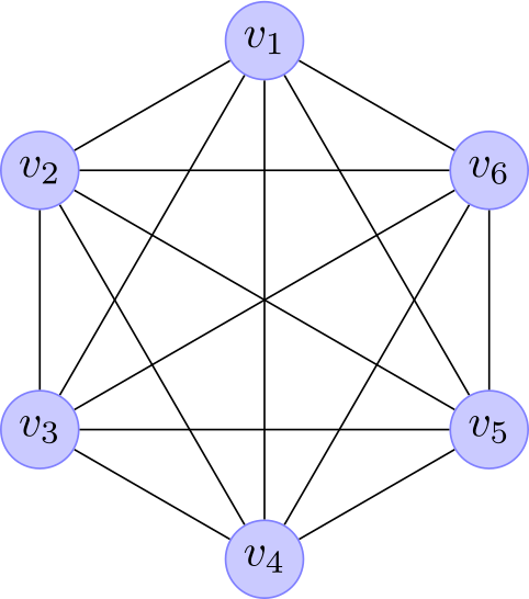
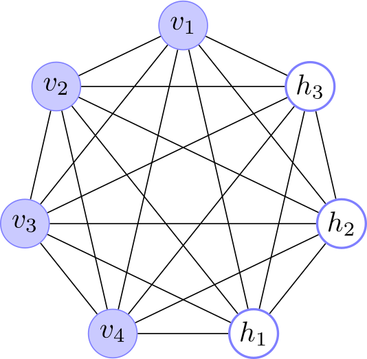
Fig. 1. Boltzmann Machine architectures. (left) A simple Boltzmann machine with only visible units. (right) A Boltzmann machine with visible and hidden units.
Activity rule
The activity rule of unit \(i\) is given by
\[\begin{equation} x_i=\begin{cases} 1 & \text{if } U[0,1] < \displaystyle\frac{1}{1+e^{-a_{i}}} \\ 0 & \text{otherwise} \end{cases} \end{equation}\]where \(a_{i}\) is the activation of unit \(i\) defined as \(a_{i}=\sum_{j}w_{ij}x_{j}\).
Learning
The process for learning the weights \(w_{ij}\in\mathbf{W}\) is done by calculating the maximum likelihood of the joint probability of equation 2. I won’t bother to explain the full derivation, since it is already brilliantly explained in chapter 43 of MacKay.
Before presenting the Boltzmann Machine learning algorithm a few points must be noted:
- The maximum likelihood leads to calculate two gradients, so the algorithm is divided in two phases: positive and negative.
- Simulated annealing is used for optimization purposes and the energy difference of unit \(i\) is given by:
- It is important to notice that the activation of unit \(a_{i}=\Delta E_{i}\)
\[\begin{equation} \Delta E_{i}=(E_{x_{i}=1}-E_{x_{i}=0})=\sum_{j}w_{ij}x_{j} \end{equation}\] - It is called Boltzmann machine since the Boltzmann distribution is sampled, but other distributions were used such as the Cauchy.
- Contrary to the Hopfield network, the visible units are fixed or clamped into the network during learning. This might be thought as making unidirectional connections between units.
- The weight update is a form of the Hebb rule learning.
- The convergence of the algorithm gets slower as more units are used.
- The annealing parts of the learning algorithm can be seen as a Gibbs sampling procedure.
There is no standard pseudocode for the Boltzmann machine, since it was not originally specified in Ackley, Hinton, and Sejnowski. I present here a compiled version I took from different books as said in the reference section. The next algorithm is for Boltzmann machines with input and output nodes, but it can be used for networks with only input units by treating all of them as output units.
While \(\mathbf{W}\) continues to change do:
Positive phase (Awake):
For each training pattern \(\mathbf{x}\):
Set the visible units equal to \(\mathbf{x}\) and clamp their values (fix the input and output nodes).
Randomly set the values for the hidden units.
Anneal:
For each decreasing temperature \(t\) in the annealing schedule:
For each epoch in the annealing schedule:
Propagate:
For \(u=1\) to number of unclamped units:
Randomly select an unclamped unit \(i\)
Calculate its energy difference \(\Delta E_{i}=\sum_{j}w_{ij}x_{j}\)
if \(U[0,1] < \displaystyle\frac{1}{1+e^{-\frac{\Delta E_{i}}{t}}}\) then:
Set \(x_i = 1\)
else:
Set \(x_i = 0\)
Collect statistics:
Set the sum co-occurance matrix \(\mathbf{S}=0\)
Set the value of temperature \(t\)
For each epoch in the annealing schedule:
Propagate:
For \(u=1\) to number of unclamped units:
Randomly select an unclamped unit $i$
Calculate its energy difference \(\Delta E_{i}=\sum_{j}w_{ij}x_{j}\)
if \(U[0,1] < \displaystyle\frac{1}{1+e^{-\frac{\Delta E_{i}}{t}}}\) then:
Set \(x_i = 1\)
else:
Set \(x_i = 0\)
Sum co-occurance of active states:
For each pair of connected units:
Set \(s_{ij} = s_{ij} + x_{i}x_{j}\)
Set each \(p^{+}_{ij}\) equal to the average of \(s_{ij}\) over all training runs and patterns
Negative phase (Sleep or Free-running):
Randomly set the values of all units.
Anneal:
For each decreasing temperature \(t\) in the annealing schedule:
For each epoch in the annealing schedule:
Propagate:
For \(u=1\) to number of unclamped units:
Randomly select an unclamped unit \(i\)
Calculate its energy difference \(\Delta E_{i}=\sum_{j}w_{ij}x_{j}\)
if \(U[0,1] < \displaystyle\frac{1}{1+e^{-\frac{\Delta E_{i}}{t}}}\) then:
Set \(x_i = 1\)
else:
Set \(x_i = 0\)
Collect statistics:
Set the sum co-occurance matrix \(\mathbf{S}=0\)
Set the value of temperature \(t\)
For each epoch in the annealing schedule:
Propagate:
For \(u=1\) to number of unclamped units:
Randomly select an unclamped unit \(i\)
Calculate its energy difference \(\Delta E_{i}=\sum_{j}w_{ij}x_{j}\)
if \(U[0,1] < \displaystyle\frac{1}{1+e^{-\frac{\Delta E_{i}}{t}}}\) then:
Set \(x_i = 1\)
else:
Set \(x_i = 0\)
Sum co-occurance of active states:
For each pair of connected units:
Set \(s_{ij} = s_{ij} + x_{i}x_{j}\)
Set each \(p^{-}_{ij}\) equal to the average of \(s_{ij}\) over all training runs
Update weights:
Modify each weight \(w_{ij}\) by \(\Delta w_{ij}=\eta(p^{+}_{ij}-p^{-}_{ij})\) where \(\eta\) is a small constant.
Recall
The recall process is just simply annealing as shown below.
Randomly set the values of the hidden and output units.
Anneal:
For each decreasing temperature \(t\) in the annealing schedule:
For each epoch in the annealing schedule:
Propagate:
For \(u=1\) to number of unclamped units:
Randomly select an unclamped unit \(i\)
Calculate its energy difference \(\Delta E_{i}=\sum_{j}w_{ij}x_{j}\)
if \(U[0,1] < \displaystyle\frac{1}{1+e^{-\frac{\Delta E_{i}}{t}}}\) then:
Set \(x_i = 1\)
else:
Set \(x_i = 0\)
Get the values of the output units.
4-2-4 Encoder problem
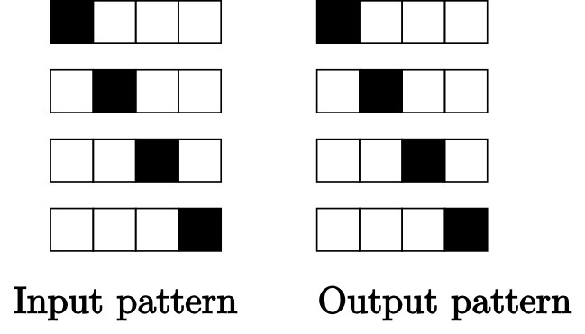
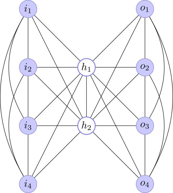
The encoder problem was originally used by Ackley, Hinton, and Sejnowski to demonstrate the learning capabalities on a “recurring task of communicating information among various components of a parallel network”. The 4-2-4 version of the problem consists in given the architecture shown in Fig. 2 learn the patterns that appear in Fig. 3.
 |
| Fig. 2. The Boltzmann Machine architecture for the 4-2-4 encoder. |
 |
| Fig. 3. The Boltzmann Machine architecture for the 4-2-4 encoder. |
The original annealing schedule setup used by Ackley, Hinton, and Sejnowski is shown in table 1. Additionally, the co-occurance sum was done for 10 epochs at a temperature equal to 10. It is also reported that they train the network 250 different times, and that the longest learning was 1810, but the median was 110.
During the positive phase, a noisy version of the input pattern was used in order to avoid the weights growing too large. Each state remained with the same value with a probability 0.85 and 0.95 for the on and off states, respectively. Finally, the weight \(w_{ij}\) was modified by \(\Delta w_{ij}=2\cdot\text{sign}(p^{+}_{ij}-p^{-}_{ij})\)
| Temperature | Num. of epochs |
| 20 | 2 |
| 15 | 2 |
| 12 | 2 |
| 10 | 4 |
Code
I programmed the 4-2-4 example mostly on the description provided by Fausset and Freeman and used the parameters given by Ackley, Hinton, and Sejnowski. On most of the cases, the recalling process was succesful for each input.
#!/usr/bin/env python

from __future__ import division
from enum import Enum
import numpy as np


Clamp = Enum('Clamp', 'VISIBLE_UNITS NONE INPUT_UNITS')

class Step:
    def __init__(self, temperature, epochs):
        self.temperature = temperature
        self.epochs = epochs

numInputUnits = 4
numOutputUnits = 4
numHiddenUnits = 2

numVisibleUnits = numInputUnits + numOutputUnits
numUnits = numVisibleUnits+numHiddenUnits

annealingSchedule = [Step(20.,2),
                     Step(15.,2),
                     Step(12.,2),
                     Step(10.,4)]

coocurranceCycle = Step(10.,10)

weights = np.zeros((numUnits,numUnits))
states = np.zeros(numUnits)
energy = np.zeros(numUnits)

connections = np.zeros((numUnits,numUnits), dtype=np.int)
for i in xrange(numInputUnits):
    for j in xrange(i+1,numInputUnits):
        connections[i,j] = 1
    for j in xrange(1,numHiddenUnits+1):
        connections[i,-j] = 1

for i in xrange(numOutputUnits):
    for j in xrange(i+1,numOutputUnits):
        connections[i+numInputUnits,j+numInputUnits] = 1
    for j in xrange(1,numHiddenUnits+1):
        connections[i+numInputUnits,-j] = 1

for i in xrange(numHiddenUnits,0,-1):
    for j in xrange(i-1,0,-1):
        connections[-i,-j] = 1

valid = np.nonzero(connections)
numConnections = np.size(valid[0])
connections[valid] = np.arange(1,numConnections+1)
connections = connections + connections.T - 1

def propagate(temperature, clamp):
    global energy, states, weights

    if clamp == Clamp.VISIBLE_UNITS:
        numUnitsToSelect = numHiddenUnits
    elif clamp == Clamp.NONE:
        numUnitsToSelect = numUnits
    else:
        numUnitsToSelect = numHiddenUnits + numOutputUnits

    for i in xrange(numUnitsToSelect):
        # Calculating the energy of a randomly selected unit
        unit=numUnits-np.random.randint(1,numUnitsToSelect+1)
        energy[unit] = np.dot(weights[unit,:], states)

        p = 1. / (1.+ np.exp(-energy[unit] / temperature))
        states[unit] = 1. if  np.random.uniform() <= p else 0

def anneal(annealingSchedule, clamp):
    for step in annealingSchedule:
        for epoch in xrange(step.epochs):
            propagate(step.temperature, clamp)

def sumCoocurrance(clamp):
    sums = np.zeros(numConnections)
    for epoch in xrange(coocurranceCycle.epochs):
        propagate(coocurranceCycle.temperature, clamp)
        for i in xrange(numUnits):
            if(states[i] == 1):
                for j in xrange(i+1,numUnits):
                    if(connections[i,j]>-1 and states[j] ==1):
                        sums[connections[i,j]] += 1
    return sums

def updateWeights(pplus, pminus):
    global weights
    for i in xrange(numUnits):
        for j in xrange(i+1,numUnits):
            if connections[i,j] > -1:
                index = connections[i,j]
                weights[i,j] += 2*np.sign(pplus[index] - pminus[index])
                weights[j,i] = weights[i,j]

def recall(pattern):
    global states

    # Setting pattern to recall
    states[0:numInputUnits] = pattern

    # Assigning random values to the hidden and output states
    states[-(numHiddenUnits+numOutputUnits):] = np.random.choice([0,1],numHiddenUnits+numOutputUnits)

    anneal(annealingSchedule, Clamp.INPUT_UNITS)

    return states[numInputUnits:numInputUnits+numOutputUnits]

def addNoise(pattern):
    probabilities = 0.8*pattern+0.05
    uniform = np.random.random(numVisibleUnits)
    return (uniform < probabilities).astype(int)


def learn(patterns):
    global states, weights

    numPatterns = patterns.shape[0]
    trials=numPatterns*coocurranceCycle.epochs
    weights = np.zeros((m,m))

    for i in xrange(1800):
        # Positive phase
        pplus = np.zeros(numConnections)
        for pattern in patterns:

            # Setting visible units values (inputs and outputs)
            states[0:numVisibleUnits] = addNoise(pattern)

            # Assigning random values to the hidden units
            states[-numHiddenUnits:] = np.random.choice([0,1],numHiddenUnits)

            anneal(annealingSchedule, Clamp.VISIBLE_UNITS)
            pplus += sumCoocurrance(Clamp.VISIBLE_UNITS)
        pplus /= trials

        # Negative phase
        states = np.random.choice([0,1],numUnits)
        anneal(annealingSchedule, Clamp.NONE)
        pminus = sumCoocurrance(Clamp.NONE) / coocurranceCycle.epochs

        updateWeights(pplus,pminus)


patterns = np.array([[1, 0, 0, 0, 1, 0, 0, 0],
                     [0, 1, 0, 0, 0, 1, 0, 0],
                     [0, 0, 1, 0, 0, 0, 1, 0],
                     [0, 0, 0, 1, 0, 0, 0, 1]])
learn(patterns)
print weights

print recall(np.array([1, 0, 0, 0]))
Listing of Simulated Annealing pseudocode.
Remarks
Although theoretically very powerful, the Boltzmann machines were not widely used since its learning process becomes slower as more units are employed. Many attempts to make it faster were done such as the mean-field annealing. It took more than two decades of research to find a practical method for learning that is currently as deep learning.
Recommendations
When I started writing this series of posts I did not have in mind the full picture of the Boltzmann machine. The information about Boltzmann Machine is not so easily available on the web (although there is a lot information on restricted Boltzmann Machines).
If you really want to understand the Boltzmann machine in depth you should know first the following:
- If you are new to Machine Learning you should check out the different types of learning in Mathematical Monk's Generative vs. Discriminative and especially in the Big Picture.
- The Hopfield network (chapter 42 of MacKays and perhaps its generalization: the Bidirectional Associative Memory (BAM) network.
- Markov random fields (to have a basic idea you could read the first part of Barber).
- The Boltzman distribution (as in the simulated annealing post read Molecular Driving Forces Statistical Thermodynamics In Chemistry And Biology).
- Gibbs sampling and simulated annealing.
- The Boltzmann machine (chapter 43 of MacKays for the theory and section 7.2.2 of Fausset).
References
For the introductory paragraph I mainly used chapter 13 of the Gallant’s book, that is freely available for members of the MIT CogNet. For the rest of the presentation of the Boltzmann machine I used chapter 43 of MacKays.
Since there is no standard learning algorithm for the Boltzmann Machines, I used different old books on neural networks. The pseudocode and the Python program is based on importance order on: Fausset, Freeman, Ackley, Hinton, and Sejnowski, Gallant, Haykin, and Mehrotra.
This post is Open Content under the CC BY-NC-SA 3.0 license. Source code in this tutorial is distributed under the Eclipse Public License.