Self-Organizing Maps
The Self-Organizing Map (SOM) is a neural network proposed by Teuvo Kohonen in 1982, also called Kohonen networks. This kind of network is employed for clustering and also for visualization purposes.
In the SOM, the neurons or cells are usually placed in a regular grid. The neural network are competitively trained in such a way that each neuron maps data items that are the most similar to it. After training, the cells that are similar between each other are located next to each other, thus forming neighborhoods. This property preserves the topology of the original input space into the grid or lattice.
Architecture
The input of the SOM is a \(m\) dimensional vector \(x\) and the output layer is formed by a lattice of \(y_{j}\) for \(j=1,\ldots,n\) neurons. Each output neuron \(y_j\) has an \(m\) dimensional weight vector \(w_j\). A SOM network with 15 output and 4 input neurons is shown in Fig. 1.
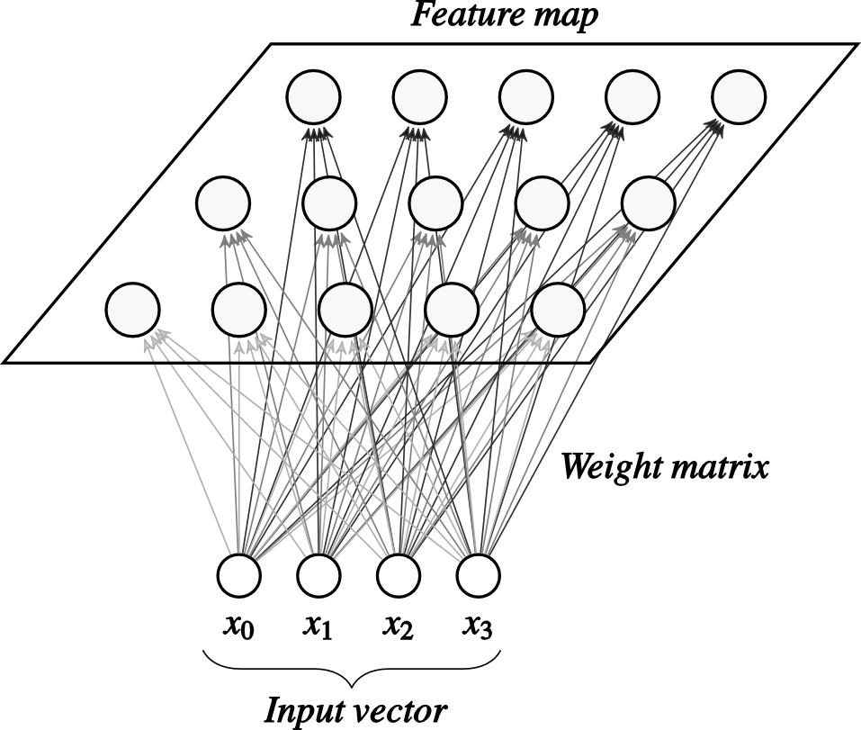 |
| Fig. 1. Architecture of a SOM network. |
Learning
The next pseudocode listing presents an online version of the SOM training algorithm. I’ll give more and specific details in the code section.
For each epoch \(t=1\) to the number of epochs:
Calculate \(\sigma(t)=\sigma_{0}exp\bigg(-\dfrac{t}{\tau}\bigg)\), where \(\sigma_{0}\) and \(\tau\) are constants.
Compute the neighborhood \(h_{i,j}(t)=exp\bigg(-\dfrac{d_{i,j}^2}{2\sigma(t)^{2}}\bigg)\) between the cells \(i\) and \(j\) for all of them.
For each pattern \(x\) in the set of randomly permuted patterns:
Calculate the output function \(y_j(x)= \parallel x-w_j \parallel\) for \(j=1,\ldots, n\)
Obtain the winning neuron \(i(x) = \displaystyle\arg \min_{\substack{j}} y_{j}(x)\), \(j=1, \ldots, n\)
Update the weight \(w_{j}(t+1) = w_{j}(t)+\eta h_{i(x),j}(t)(x-w_j(t))\) for \(j=1, \ldots, n\)
RGB color space problem
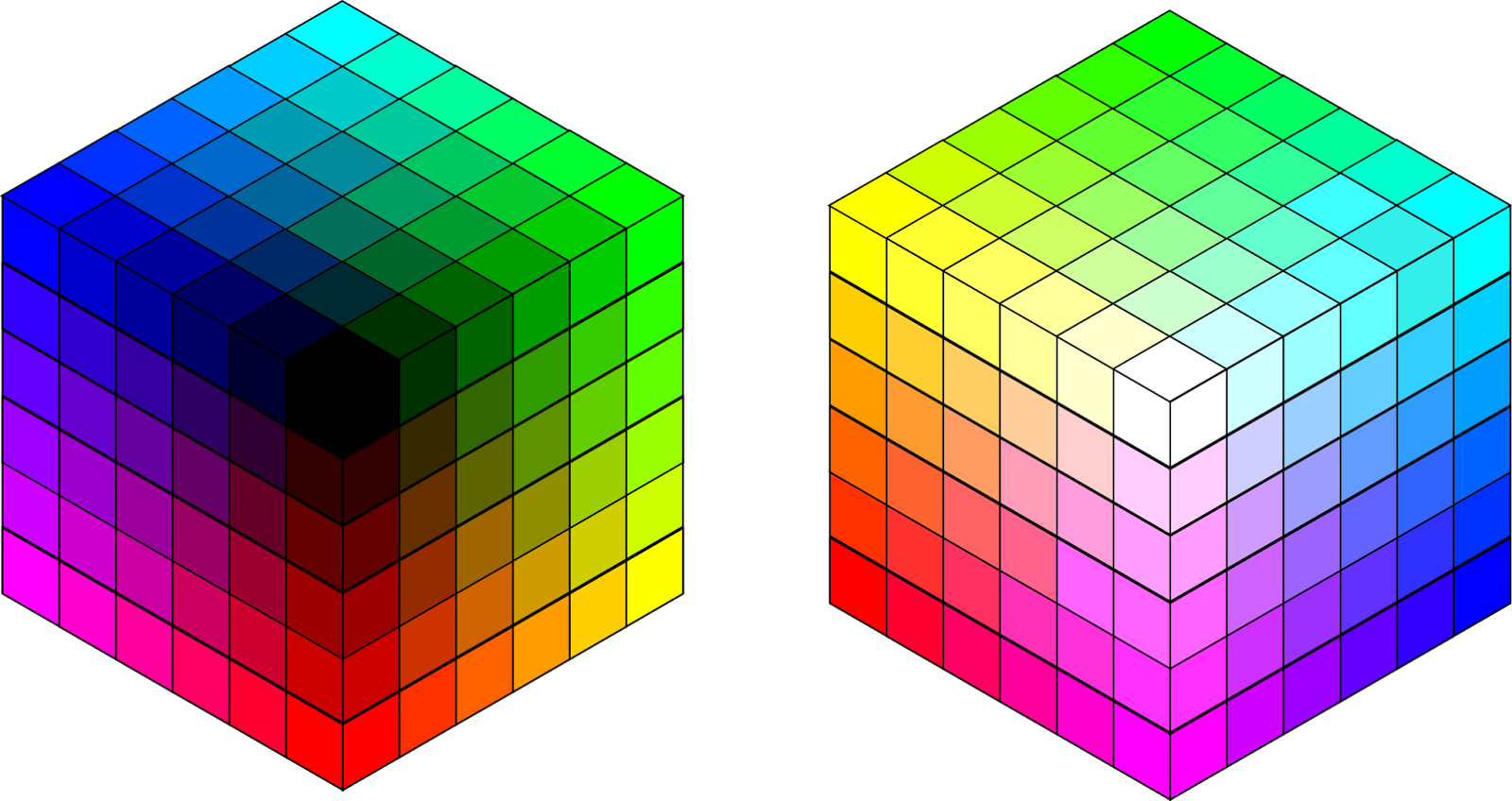
The Red Green Blue (RGB) color space is an additive color space commonly use in computer graphics. In this space, a color is represented by a three-dimensional vector containing the intensities of the color red, green, and blue. One way to represent a color intensity is to set its value between 0 and 1. Therefore, color space forms a cube as seen in Fig. 2.
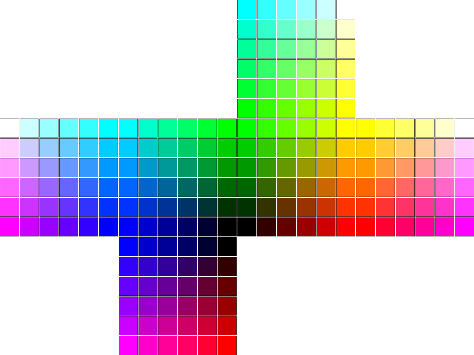
Our toy problem is to map the three-dimensional space into a bidimensional space. A simple solution is to unfold the six faces of the cube into planar views as shown in Fig. 3.
We can solve this problem using a Kohonen network by setting its inputs as random samples of the color space. The resulting weight matrix will have three-dimensional vectors that can be plotted as colors. The solution and the final map will be present in the next section.
Code
This is the first post that I wrote using IPython Notebook, so some code lines like the following are specifically for it.
The protocol stuff comes first, so let’s use matplotlib inline
matplotlib inline
and load the necessary libraries
#!/usr/bin/env python
from __future__ import division

import numpy as np
import matplotlib.pyplot as plt
import matplotlib.patches as mpatches
In this example, each weight represents a color distributed along a rectangular grid. So we need a function to plot our desired grid or map of weights.
def plotMap(colors, numRows, numCols):
    # Plotting squares
    plt.figure(figsize=(1,1))
    squareSide = 0.2

    size = 5
    if numCols > numRows:
        ax = plt.axes([0,0,size,size/(numCols*squareSide)])
        plt.axis((0,numCols*squareSide,0,numRows*squareSide))
    elif numCols < numRows:
        ax = plt.axes([0,0,size,size/(numRows*squareSide)])
        plt.axis((0,numRows*squareSide,0,numCols*squareSide))
    else:
        ax = plt.axes([0,0,size,size])
        plt.axis((0,numRows*squareSide,0,numCols*squareSide))

    for i in xrange(numRows*numCols):
        coords = squareSide*np.array([np.floor(i/numRows), (numCols-1-i)%numCols])
        color = tuple(colors[i,:])
        square = mpatches.Rectangle(coords, squareSide, squareSide, color = color, linewidth=0.5)
        plt.gca().add_patch(square)

    ax = plt.gca()
    xticks = [str(int(np.round(tick))) for tick in np.arange(0,numCols+1,numCols/(len(ax.get_xticklabels())-1))]
    yticks = [str(int(np.round(tick))) for tick in np.arange(0,numRows+1,numRows/(len(ax.get_yticklabels())-1))]
    ax.set_xticklabels(xticks)
    ax.set_yticklabels(yticks)
The neighborhood of a grid is defined by its cell shape, they not only can be rectangular but also hexagonal and form structures like honeycombs. The code only works with rectangular cells since it is faster and easier to work than with hexagonal cells.
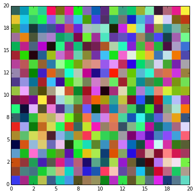
We must define the map of weights \(w_j\) and its outputs \(y_j\), where \(j = 1,\ldots, n\) and \(n\) is the number of cells. Initially, we can define a 20x20 map of random weights \(w_{j}\) that multiply a three-dimensional vector input \(x\) representing a RGB color.
numRows = 20
numCols = 20
numInputs = 3
numOutputs = numRows*numCols

outputs = np.zeros((numOutputs,1))
weights = np.random.uniform(size=(numOutputs,numInputs))
Clearly, our first map is an arrange of random colors.
plotMap(weights,numRows,numCols)
plt.show()
For the sake of optimization, lets calculate the constant squared Euclidean distance between each cell given by \(d_{i,j}^2=(j_1-i_1)^2+(j_2-i_2)^2\)
cols = np.arange(numOutputs)%numCols
rows = np.floor(np.arange(numOutputs)/numCols).astype('int')

sqrDistance = np.zeros((numOutputs,numOutputs))
for i in xrange(numOutputs):
    sqrDistance[i,:] = np.power(rows-rows[i],2) + np.power(cols-cols[i],2)
Before introducing the SOM training function, it is necessary to declare the functions that control how the neighborhoods and the weights shrink and update at each epoch, respectively. The neighborhood \(h_{i,j}\) between the cells \(i\) and \(j\) is given by the Gaussian function:
\(h_{i,j}(t)=exp\big(-\dfrac{d_{i,j}^2}{2\sigma(t)^{2}}\big)\)
and
\(\sigma(t)=\sigma_{0}exp\big(-\dfrac{t}{\tau}\big)\)
where \(t\) is the epoch number and \(\sigma_{0}\) and \(\tau\) are constants. Lets declare the value of these three last constants:
epochs = 200

sigma0 = 1.35
tau = 200
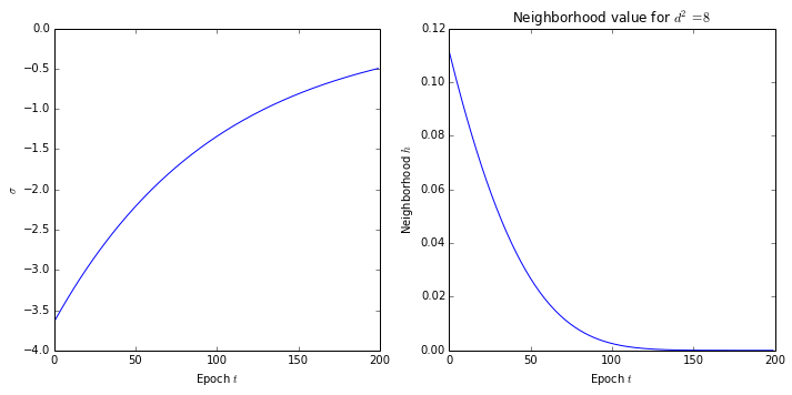
We can plot how the neighborhood for a constant distance shrinks during the training with the following:
t = np.arange(epochs)
sigma = -2*np.power(sigma0*np.exp(-t/tau),2)
neighborhood = np.exp(8/sigma)

fig = plt.figure(figsize=(1,1))
fig.set_size_inches(10, 5)

plt.subplot(1,2,1)
plt.plot(t, sigma)
plt.xlabel('Epoch $t$')
plt.ylabel('$\sigma$')

plt.subplot(1,2,2)
plt.plot(t, neighborhood)
plt.xlabel('Epoch $t$')
plt.ylabel('Neighborhood $h$')
plt.title('Neighborhood value for $d^2=8$')

plt.tight_layout()
plt.show()
The only left constant we are missing to declare is the learning rate \(\eta\), which can also be a value decaying function.
eta = 0.3
Basically, the SOM training algorithm consists of three processes: competition, cooperation, and adaptation. During the competition process, the output \(y_j\) of each cell \(j\) is calculated by
\[y_j(x)= \parallel x-w_j \parallel\]Subsequently, the winning neuron or cell \(i(x)\) is given by
\(i(x) = \displaystyle\arg \min_{\substack{j}} y_{j}(x)\), \(j=1, \ldots, n\)
The cooperation process computes the neighborhood value of the winning cell \(h_{i(x),j}(t)\) for the current epoch \(t\). The last process updates the weights values \(w_j\) for all cells by
\[w_{j}(t+1) = w_{j}(t)+\eta h_{i(x),j}(t)(x-w_j(t))\]We can declare the SOM training algorithm as
def train(patterns):
    global outputs, weights

    numPatterns = patterns.shape[0]
    for t in xrange(epochs):

        sigma = -2*np.power(sigma0*np.exp(-t/tau),2)
        neighborhood = np.exp(sqrDistance/sigma)

        for i in np.random.permutation(numPatterns):
            inputs = patterns[i,:]

            # Propagate
            outputs = np.sqrt(np.power(inputs-weights,2).sum(axis=1))
            winner = outputs.argmin()

            # Update
            weights += eta*(inputs - weights)*neighborhood[winner,:][:,None]
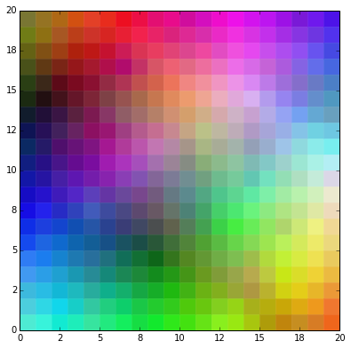
Finally, we can take a uniform distributed sample of colors from the RGB space, train the SOM with it, and plot the resulting map.
np.random.seed(seed=30)
numPatterns = 60*60
patterns = np.random.uniform(size=(numPatterns,numInputs))

train(patterns)

plotMap(weights,numRows,numCols)
plt.show()
References
I wrote this post using three books: Battiti, Haykin, and Freeman. The first book, also known as the LION book, provides a good introduction of different topics on Machine Learning and Optimization. I recommend to read it before getting on other more technical details. For writing the code, I started using Freeman’s, but a great improvement came from Freeman’s.
Another good reference I used is provided in an article written by Teuvo Kohonen for scholarpedia.
This post is Open Content under the CC BY-NC-SA 3.0 license. Source code in this tutorial is distributed under the Eclipse Public License.