Factor Analysis

Factor analysis (FA) is a latent variable model that describes the variability of a given dataset. It was developed by the psychologists Charles Spearman, Raymond Catell, and Louis Leon Thurstone.

FA tries to explain the dependencies among the observed variables in terms of a smaller number of unobserved latent variables, or factors, without loss of information. Statistically, the dependencies between variables are defined by the covariance.

It can be used for dimensionality reduction, detecting structure in the relationships between variables, and visualization purposes.

Model

The FA graph model, which is a latent variable model, appears in fig. 1.


(a)		(b)

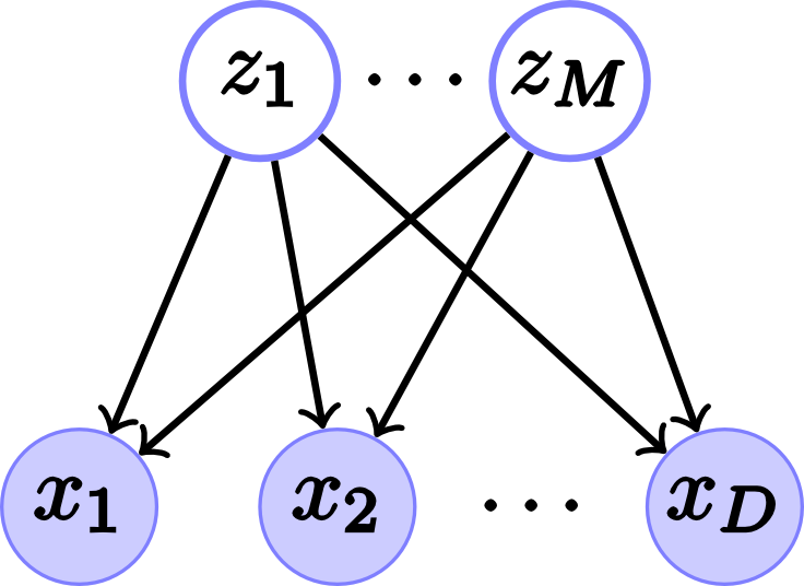
Fig. 1. Factor analysis model. (a) Belief network for $D$ visible nodes and $M$ hidden nodes or factors and its (b) Vector form.

The probability of this belief network can be expressed as:

\[p(x_1, \ldots, x_D, z_1, \ldots, z_M)=p(x_1, \ldots, x_D|z_1, \ldots, z_M)p(z_1, \ldots, z_M)\]

In vector form

\[p(\mathbf{x},\mathbf{z})=p(\mathbf{x}|\mathbf{z})p(\mathbf{z})\]

The model assumes that

The factors are unit normals, i.e. $p(z_i)=\mathcal{N}(0,1)$ for each $i=1, \ldots, m$, where $m$ is the number of factors.
They are uncorrelated, i.e. $\mathrm{Cov}(z_i, z_j)$ for $i\neq j$.

So in vector form we have that $p(\mathbf{z})=\mathcal{N}(0,I)$.
The probability $p(\mathbf{x}\vert\mathbf{z})$ is also a Gaussian distribution defined as $\mathcal{N}(\mathbf{x}\vert W\mathbf{z}+\mu,\Psi)$, where $W$ is the $D$x$M$ factor loadings matrix, $\mu$ is the mean of $x$, and the matrix $\Psi=$diag$(\psi_1, \ldots, \psi_D)$. Each column of the factor loadings matrix $W$ captures the covariance among the variables and the diagonal values of $\Psi$ are called uniquenesses.

Therefore, the probability $p(\mathbf{x})$ is a Gaussian pancake defined as:

\[p(\mathbf{x})=\int p(\mathbf{x}|\mathbf{z})p(\mathbf{z})d\mathbf{z}=\mathcal{N}(\mu,\Sigma)\]

where $\Sigma=W W^\intercal+\Psi$.

So an observation is mathematically generated by

\[\mathbf{x}=W\mathbf{z}+\mu+\epsilon\]

where $\epsilon$ represents the noise that can’t be explained by the factors and it’s defined as $\mathcal{N}(0,\Psi)$

Learning $W$ and $\Psi$

$W$ and $\Psi$ can be learned using Principal Factor Analysis (see Mardia), Maximum Likelihood or the Expectation Maximization (EM) algorithm (both appear in detail in Barber). In this post I implemented the EM algorithm by following the description and equations in Bishop. The aim of the E-step is to infer $p(\mathbf{z}\vert x_i)$ for each $x_i$ by:

$\mathbb{E}\big[\mathbf{z}^{(n)}\big]=\mathbf{G}W^\intercal\Psi^{-1}(\mathbf{x}^{(n)}-\overline{\mathbf{x}})$ $\mathbb{E}\big[\mathbf{z}^{(n)}{\mathbf{z}^{(n)}}^\intercal\big]=\mathbf{G}+\mathbb{E}\big[\mathbf{z}^{(n)}\big]\mathbb{E}\big[\mathbf{z}^{(n)}\big]^\intercal$

where $\mathbf{G}=\mathbf{I}+(W^\intercal\Psi^{-1}W)^{-1}$.

In the M-step a linear regression from $\mathbf{z}$ to $\mathbf{x}$ to get $W$ is performed:

\[W^{new}=\bigg[\sum^{N}_{n=1}(\mathbf{x}^{(n)}-\overline{\mathbf{x}})\mathbb{E}\big[\mathbf{z}^{(n)}\big]\bigg]\bigg[\sum^{N}_{n=1}\mathbb{E}\big[\mathbf{z}^{(n)}{\mathbf{z}^{(n)}}^\intercal\big]\bigg]^{-1}\] \[\Psi^{new}=\text{diag}\bigg\{\mathbf{S}-W^{new}\frac{1}{N}\sum^{N}_{n=1}\mathbb{E}\big[\mathbf{z}^{n}\big](\mathbf{x}^{(n)}-\overline{\mathbf{x}})^{\intercal}\bigg\}\]

where $\mathbf{S}=\frac{1}{N}\sum_{n=1}^{N}(\mathbf{x}^{(n)}-\overline{\mathbf{x}})(\mathbf{x}^{(n)}-\overline{\mathbf{x}})^\intercal$ is the covariance of the sampled data.

Likelihood

The log likelihood of a given dataset $\mathbf{X}=(\mathbf{x}^{(1)}, \ldots, \mathbf{x}^{(N)})$ for FA is simply the log likelihood of a multivariate normal distribution:

\[\begin{aligned} \ln p(\mathbf{X}|\mu,\Sigma) & = \ln\prod_{n=1}^{N}\mathcal{N}(\mathbf{x}^{(n)}|\mu,W W^\intercal+\Psi) \\ & = -\frac{N D}{2}\ln(2\pi)-\frac{N}{2}\ln \det(\Sigma)-\frac{1}{2}\prod_{n=1}^{N}(\mathbf{x^{(n)}}-\mu)^\intercal \Sigma^{-1}(\mathbf{x^{(n)}}-\mu) \end{aligned}\]

By differentiating the last equation with respect to $\mu$ and equating to zero, we obtain the mean of the observed data points:

\[\mu=\frac{1}{N}\sum_{n=1}^{N}\mathbf{x^{(n)}}=\overline{\mathbf{x}}\]

Using this result, the log likelihood can be written as

\[\ln p(\mathbf{X}|\mu,\Sigma)=-\frac{N}{2}\big(D\ln2\pi+\ln\det(\Sigma)+\text{trace}(\Sigma^{-1}\mathbf{S})\big)\]

The code for the Factor Analysis EM algorithm is as follows:

#!/usr/bin/env python
from __future__ import division

import numpy as np
from numpy import linalg as la

def factorAnalysis(x, numFactors, numIterations):    
    numData, numDim = x.shape
    mu = x.mean(axis=0)
    x -= mu
    
    cov =(x.T*x)/numData

    I = np.eye(numFactors)
    Psi = np.diag(np.diag(cov))
    scaling = np.power(la.det(cov), 1./numData)
    W = np.random.normal(0,np.sqrt(scaling/numFactors),(numDim,numFactors))

    oldL = -np.inf
    for i in xrange(numIterations):
        
        # Expectation step
        WPsi = np.dot(W.T,la.pinv(Psi)) 
        G = la.pinv(I+np.dot(WPsi,W))
    
        ez = np.dot(G,np.dot(WPsi,x.T)) 
        ezz = numData*G+np.dot(ez,ez.T)
    
        # Maximization step
        xEz = np.dot(x.T,ez.T)
        W = xEz*la.pinv(ezz)
        Psi = np.diag(np.diag(cov-np.dot(W,xEz.T)/numData))
        
        # Log Likelihood
        Sigma = W*W.T + Psi
        logSigma = np.log(la.det(Sigma))
        L = -numData/2*(np.trace(la.pinv(Sigma)*cov.T)+numDim*np.log(2*np.pi)+logSigma)
        
        if (L-oldL)<(1e-6):
            break
        oldL = L
        
    return W, Psi, mu

Interpretability and Factor rotation

The factor loadings matrix $W$ is not a unique solution, since other valid solutions can be found by multiplying it by orthogonal matrices (i.e. $\mathbf{R}\mathbf{R}^\intercal=I$). In other words, the variance $\Sigma$ of $p(\mathbf{x})$ is equal to

\[(W\mathbf{R})(W\mathbf{R})^\intercal+\Psi=W\mathbf{R}\mathbf{R}^\intercal W^{\intercal}+\Psi=WIW^{\intercal}+\Psi=WW^{\intercal}+\Psi\]

If we wish to find a more interpretable $W$, we must seek a rotation matrix $\mathbf{R}$ that makes $W$ to have columns with a small number of large values. One orthogonal method for finding a suitable rotation matrix is Varimax. The next Varimax rotation algorithm is taken from a wikipedia talk.

def varimax(Phi, gamma = 1.0, q = 20, tol = 1e-6):
    from numpy import eye, asarray, dot, sum, diag
    from numpy.linalg import svd
    p,k = Phi.shape
    R = eye(k)
    d=0
    for i in xrange(q):
        d_old = d
        Lambda = dot(Phi, R)
        u,s,vh = svd(dot(Phi.T,asarray(Lambda)**3 - (gamma/p) * dot(Lambda, diag(diag(dot(Lambda.T,Lambda))))))
        R = dot(u,vh)
        d = sum(s)
        if d_old!=0 and d/d_old < 1 + tol: break
    return dot(Phi, R)

Dimensionality reduction

The dimensionality reduction works when the number of factors $M$ is less than the number of dimensions $D$. We can find the values of $\mathbf{Z}$ by following a multivariate linear regression approach, as Alpaydin. So we would like to find $\mathbf{z}^{(i)}$ for each observation $i\in 1, \ldots, N$ such that

\[\mathbf{z}^{(i)}=\mathbf{V}^{\intercal}(\mathbf{x}^{(i)}-\overline{\mathbf{x}})+\mathbf{\epsilon}\]

where $\mathbf{V}$ have unknown values and $\mathbf{\epsilon}$ is zero-mean noise. By applying a transponse operation to the last equation over all observations, we have

\[\mathbf{Z}=\overline{\mathbf{X}}\mathbf{V}+\mathbf{\Xi}\]

where $\overline{\mathbf{X}}=\mathbf{X}-\overline{\mathbf{x}}$. This is a multivariate linear regression that it solved by:

\[\mathbf{Z}=\overline{\mathbf{X}}\mathbf{V}=\overline{\mathbf{X}}(WW^{\intercal}+\Psi)^{-1}W\]

Example

The data from this example is taken from the Open/Closed book examination problem from Mardia et al. The data consists of the test scores of 88 students on 5 subjects (Mechanics, Vectors, Algebra, Analysis, and Statistics). The first two columns of data correspond to closed book examinations, while the rest to opened book examinations. If the number of factors $M$ is set to two, then we get the graphical model that appears in Fig. 2.

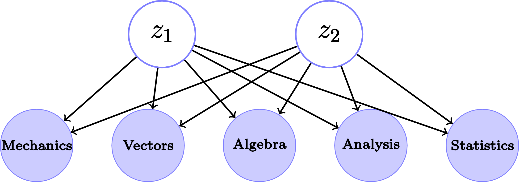
Fig. 2. Graphical model for the Open/Closed book examination data for $M=2$.

Before starting is important to say that I originally used iPython throughout the example. First, lets load the data and display it

# Loading the Open/Closed book test scores data
scores = np.asmatrix(np.genfromtxt("http://www-eio.upc.es/~jan/Data/BookOpenClosed.dat",delimiter="\t",skiprows=1))

# Format the data output
import sympy as sp
sp.init_printing()
sp.Matrix(scores[0:10,:])

$$\left[\begin{matrix}77.0 & 82.0 & 67.0 & 67.0 & 81.0\\63.0 & 78.0 & 80.0 & 70.0 & 81.0\\75.0 & 73.0 & 71.0 & 66.0 & 81.0\\55.0 & 72.0 & 63.0 & 70.0 & 68.0\\63.0 & 63.0 & 65.0 & 70.0 & 63.0\\53.0 & 61.0 & 72.0 & 64.0 & 73.0\\51.0 & 67.0 & 65.0 & 65.0 & 68.0\\59.0 & 70.0 & 68.0 & 62.0 & 56.0\\62.0 & 60.0 & 58.0 & 62.0 & 70.0\\64.0 & 72.0 & 60.0 & 62.0 & 45.0\end{matrix}\right]$$

Now lets call the factor analysis algorithm for the case $M=2$.

np.random.seed(20)
[W, Psi, mu] = factorAnalysis(scores, 2, 1000)

Lets format and output the factor loadings matrix:

from pandas import DataFrame
DataFrame(W,index=['Mechanics','Vectors','Algebra','Analysis','Statistics'], columns=['$\mathbf{w}_1$','$\mathbf{w}_2$'])

	$$\mathbf{w}_1$$	$$\mathbf{w}_2$$
Mechanics	-2.900648	-12.359802
Vectors	-1.179214	-9.899666
Algebra	3.349823	-8.907011
Analysis	6.278075	-10.090045
Statistics	7.012489	-10.878233

We can interpret the first factor as a contrast between the first two variables and the rest, which correspond to the closed book examination problem. The values of the second factor are almost the same, suggesting a weighted average of the variables. The latter interpretation might not be clear due the negative sign of the factors, but we can rotate the factor loadings matrix by $180^\circ$ or $\mathbf{R}=-\mathbf{I}$.

Now we can rotate the factor loadings matrix using the varimax algorithm, and thus changing the interpretation.

WR = varimax(W)
DataFrame(WR,index=['Mechanics','Vectors','Algebra','Analysis','Statistics'], columns=['$\mathbf{w}_1$ (rotated)','$\mathbf{w}_2$ (rotated)'])

	$$\mathbf{w}_1$$ (rotated)	$$\mathbf{w}_2$$ (rotated)
Mechanics	4.915857	-11.705247
Vectors	4.863105	-8.703112
Algebra	7.944409	-5.238562
Analysis	11.008939	-4.475095
Statistics	12.066336	-4.681290

The only thing left to do in this example is to reduce the dimension of the data.

# Note: the scores have already been subtracted by the mean in the factorAnalysis function
z = np.dot(scores,la.inv(W*W.T+Psi)*W)

Notes and lots of missing things

If $\Psi=\sigma^2\mathbf{I}$ we obtain the Probabilistic Principal Component Analysis (PCA) model.
The Restricted Boltzmann Machines are the binary version of the FA model.
A roadmap to more complex dynamic models is shown in these slides.
In Mardia et. al. the algorithm used to learn $W$ is Principal Factor Analysis, but some elements of the correlation matrix are wrong,
In this post I didn’t talk about determining the number of factors $M$. In Wikipedia’s FA article is stated the criteria to set $M$, but is also said that some of them are contradictory. So you might follow a Bayesian approach.
I didn’t use FA for visualization purposes.
Another thing missing is the geometric interpretation of the FA model is missing.

Recommendations and references

If you want a simple introduction and a getting-started example you should check this post in Scientific American.
Two good complementary theory introductions are provided in Barber and Alpaydin (which is freely available for members of MIT CogNet). Additionally, you can check Ng’s handout for more details.
For programming the EM algorithm for FA I followed the equations in Bishop and got some help from the implementation in Marsland